Carrick cited Savitzky-Golay filters. I hadn't paid these much attention, but I see the relevant feature here is something that I had been using for a long time. If you want a linear convolution filter to return a derivative, or second derivative etc, just include test equations applying to some basis of powers and solve for the coefficients.
I've been writing a post on this for a while, and it has grown long, so I'll split in two. The first will be mainly on the familiar linear trends - good and bad points. The second will be on more general derivatives, with application to global temperature series.
Trends
We spend a lot of time talking about linear trends, as a measure of rate of warming (or pause etc). I've made a gadget here to facilitate that, even though I think a lot of the talk is misguided. Sometimes, dogmatic folk insist that trends should not be calculated without some prior demonstration of linear behaviour.A silly example of this came with Lord Donoughue, in the House of Lords, monstering a Minister and the MetOffice, with Doug Keenan pulling the strings. The question was a haggle over significant rise, with Keenan badgering the MO to calculate it his pet way, the MO saying (reasonably) that they don't talk much about trends, accusations of the MO using inappropriate models etc. It really isn't that hard. A trend is just a weighted sum of readings. It has the same status as any other kind of average, and it has uncertainty like that of the standard error of the mean.
Trend as derivative
But a time series trend β can be seen as just a weighted average of derivatives. To see this in integral form:β=∫xy dx/∫x² dx
where x is from -x0 to x0. Integrating by parts:
β=∫W(x0,x)y'(x) dx where W=(x0²-x²)/∫x² dx
W is a (Welch) taper which is zero at the ends of the integration range. I'll be using it more. But while it damps high frequencies, with roll-off O(1/f²) in the frequency domain, the differentiation itself brings back a factor of f, so net effect is O(1/f).
In the next post I'm looking at the effect of better noise suppression.
Trend as Savitsky operator
In my version of the Savitsky process for time series (x), I take a filter W and ask for the polynomial P that satisfies constraints∑xP(x) W(x) xi=ci
where the order of P equals the number of constraints. This is a linear system in the coefficients of P. P(x) W(x) will be the operator. For a differentiation operator, c=(0,1). You can go to higher order with c=(0,1,0,0) etc. For second derivative, c=(0,0,2).
Symmetry helps. If W is symmetric (x is centered),
P(x)= x/∑x2W
and the trend coefficient of series y is β = ∑x*yW
/ ∑x2W
If W is the boxcar filter, value 1 on a range, this is the OLS regression formula.
OLS trend as minimum variance estimator
A useful property to remember about the ordinary mean is that it is the number which, when subtracted, minimises the sum of squares. There is a corresponding property for OLS trend. It is the operator which, of all those Vi satisfyingVixi=1 (summation convention)
has minimum sum squares ViVi. That is just an orthogonality property. And since for any time series y, Viyi is the trend estimate β, the variance of that estimate is (ViVi)* var(y). So of all eligible V, the OLS trend has minimum variance.
The good and bad
So trend is a minimum variance estimate of derivative, but with poor noise damping. I'll compare next with operators where W is a quadratic taper, coming down to 0 at the ends, so continuous (Welch window). As smoother, it thus gives high frequency roll-off O(1/f2). W2 (Parzen window) then has continuous derivative, and roll-off O(1/f3).So here is a plot of the spectra, tapers centered so the spectrum is pure imaginary. The OLS trend operator is colored red, and given a 10-year period (width).
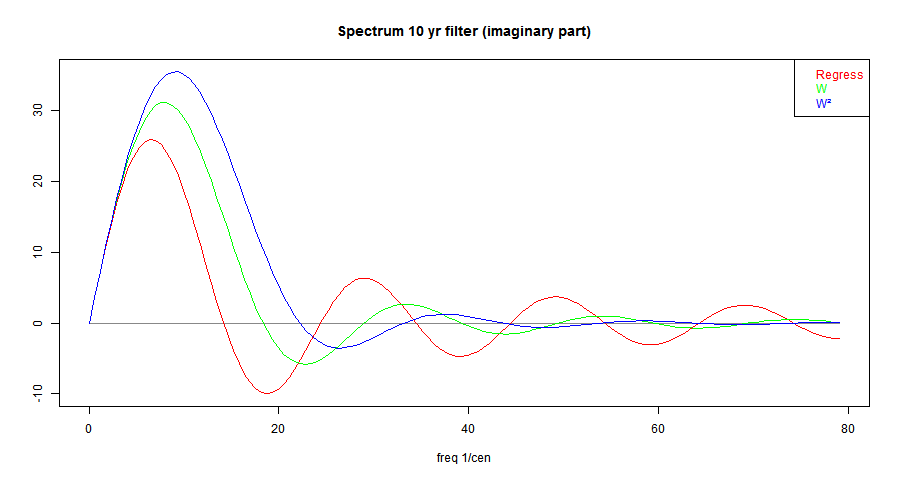
Some points:
- Each of the operators is linear for low frequencies, as differentiation requires. As the frequency (1/width) = 10 /Cen is approached, the response starts to taper. This is the effect of smoothing at higher frequencies. The smoother tapers have a later cut-off, because they are effectively narrower in the time domain.
- Each operator then has some band-pass character. This will show in their behaviour. It is an inevitable consequence of combining a linear start with a hf roll-off.
- You can see the 1/f roll-off at high frequencies, compared to the other operators. This is the bad feature of trend as a derivative. If you have decided on a cut-off, you want it to be observed. The operator is no longer differentiating properly (linear), and so is unhelpful at higher frequencies. It is best if it fades quickly.


Nick,
ReplyDeleteThe filter you mention is an example of a FIR filter, as such it 'should' have a finite response function.
http://en.wikipedia.org/wiki/Savitzky%E2%80%93Golay_filter#Treatment_of_first_and_last_points
The above suggested approach 'mirror image' is not a very good idea (at least for an end condition that is 'steep'), I usually try a double flip 'mirror image' but even there it becomes rather tricky (removing and adding a low order polynomial helps there)..
I've used FFT (removing a lower polynomial first, and forcing the polynomial through both end points), but this has issues at the lowest and transition band frequencies.
I've also used an IIR filter (two-pass Butterworth with zero padding, again removing a lower polynomial first, then adding it back afterwards, running at quad precision up to N = 80 pole count), this becomes really difficult for short time series as the filter literally rings forever (I'm 'still' working on that one).
For the IIR filter, I use a 9-point FD stencil for the 1st and 2nd derivatives.
Similarly, a FIR LOESS (n = 2 quadratic) 'can' be used (just don't do interpolation as the response is 'lumpy'), again I use a 9-point FD stencil for the 1st and 2nd derivatives.
AFAIK, all filters suffer from the end point problem inherent in finite time series (you only have half the information at the end as you do in the middle).
Don't have the necessary math skills, I always test with a very long white noise time series, chop the series up, and look at the various filter end effects.
Everett, the definition of an ideal low-pass filter is step function in the frequency response. However, this requires a theoretically infinitely long sinc fn kernel to achieve. The rest of the game is how to approach that idea in a calculable way.
DeleteIn electronics and audio, it is usual to have a continuous stream of data and so IIR solutions are often used. In image processing, as in time series analysis, kernel based FIR solutions are more appropriate.
The question is then the best way to window the sinc fn to make it finite without causing too much distortion.
The Lanczos filter is one of the best. It has a fast transition band and low ripple in stop- and pass-bands.
http://climategrog.wordpress.com/2013/11/28/lanczos-filter-script/
It has the disadvantage of requiring a rather longer kernel than other options but is a very good filter.
Nick I should mention that the problem for derivative filters is slightly easier with climate (and many related signal types) than the general problem, because the spectrum already has a 1/f^nu, nu > 1, character to it.
ReplyDeleteLike you, I don't stick with a rectangular window for general data (I typically find rectangular windows work well enough for temperature data usually). Instead, I use window functions that include Welch, Hann, Blackman and modified Gaussian (this is a tunable window, which has advantages).
I think I mean the re-trended PDO, which looks pretty much like the SAT until around 1980 to 1985, at which time it makes a prolonged excursion in another direction.
ReplyDelete"A useful property to remember about the ordinary mean is that it is the number which, when subtracted, minimises the sum of squares. There is a corresponding property for OLS trend. "
ReplyDeleteIsn't this the same as saying that OLS trend is identical to mean of dT/dt ?
"Isn't this the same as saying that OLS trend is identical to mean of dT/dt ?"
DeleteNo. As said in the recent post, trend is the Welch-weighted mean of dT/dt.
Consider the following: running mean of diff is same as diff of RM. The kernel that achieves that has just two non zero values of opposite sign, one at each end of the kernel. Its the two point diff of the rectangular RM kernel.
Delete( This is in fact the same thing as the pairs of points Pekka referred to in the other thread, I'll come back to that ).
As you have pointed out the OLS regression slope is the correlation of the data with a kernel of unit slope. If that is centred to be zero mean, the diff of that kernel is a positive rectangular window with a negative point as first and last element. These points are not unimportant and it cannot be shifted up to make it a simple rectangle.
Your Welch window applied to TS is the same as ramp applied to dT/dt and so corresponds to the OLS trend in dT/dt ie the acceleration trend that you started out discussing, not the OLS trend of the TS. Again, this cannot be arbitrarily shifted up or down.
Your integral maths was good but there is a logical error in how you interpret the terms.
Oh, no, it's my error. You were applying W to dT/dt not to TS Care needs to be taken with shifting the kernel up or down since this will be adding a constant to each element and hence adding a fixed dT/dt to the whole series.
Delete